Overview
Data augmentation is a necessary regularization technique for successfully training deep networks. For vision problems, this typically involves applying random affine-transformations, flips, crops, contrast-adjustments, and noise to input images. Recently, some have even proposed iteratively augmenting the training set with adversarial examples. For object detection, bounding boxes are also usually randomly perturbed.
Although these methods greatly expand the size of the training set, they are limited to the extent that the content of an image is not changed in any semantic or substantive way as would be perceived by a human. In this post, I outline a method for creating new training examples for object detection tasks using a technique called poisson blending. I also provide reference implementations in NumPy/SciPy.
Poisson Blending
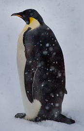
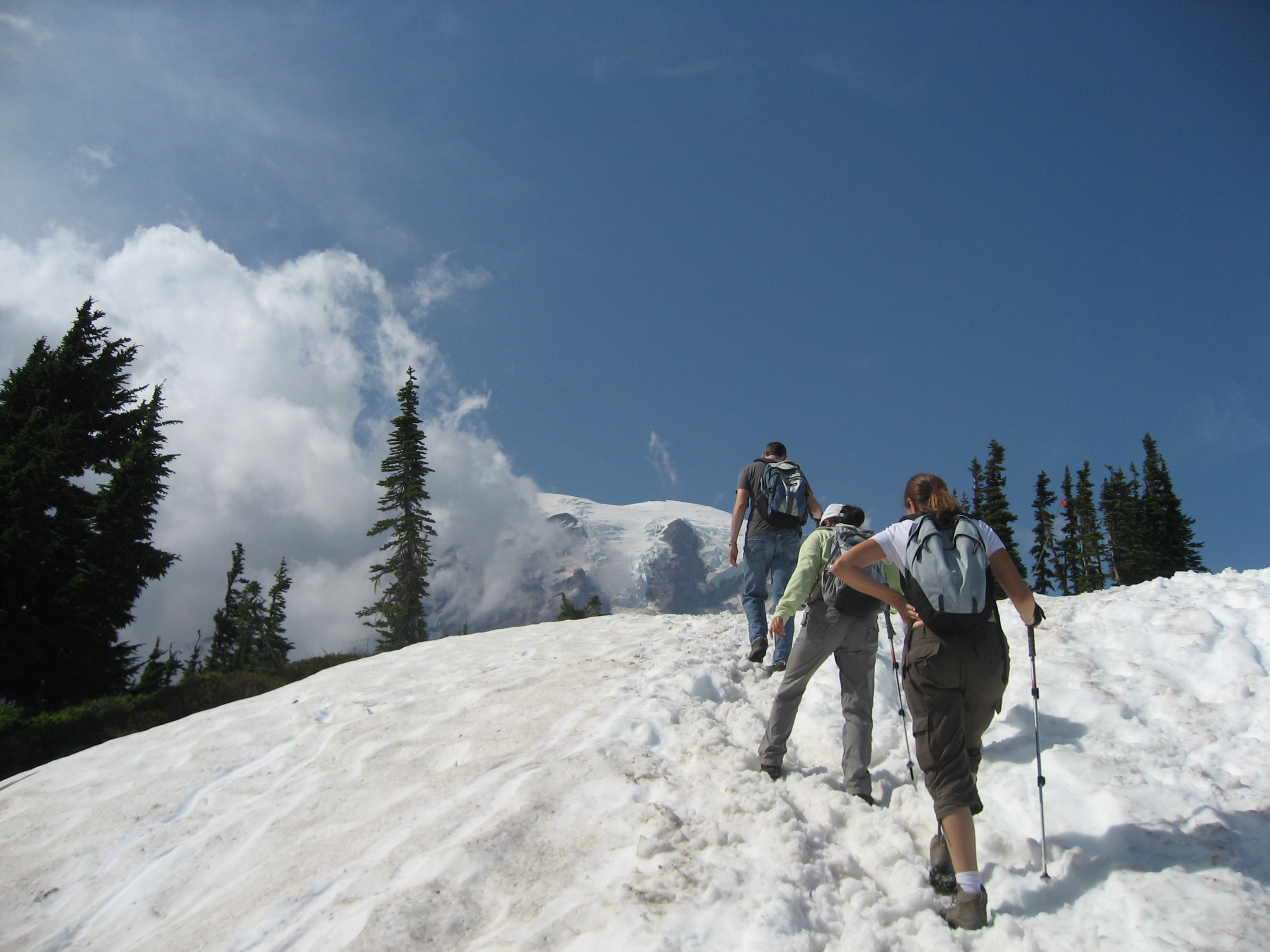
Poisson blending is a “copy-paste” method for inserting a source image \(S\) into a target image \(T\). The method is best conveyed visually. Below we have images of a penguin (the source) and a mountain (the target).
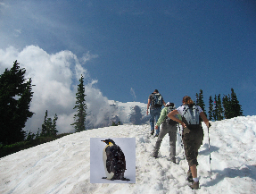
We wish to paste the penguin onto the mountain in a realistic way. Unfortunately, naively copying respective pixels from \(S\) into \(T\) yields a noticeable seam as shown below.
Poisson blending addresses this concern and would instead produce the following result.
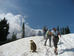
Despite a fairly loose crop around the penguin, the seam between \(S\) and \(T\) is now much harder to detect.
Poisson blending originates from the computational photography literature and belongs to a family of techniques known as gradient-domain processing. To explore how it works, let’s first define \(V\) to equal the new source pixel values that are pasted into \(T\). Poisson blending exploits the observation that preserving image gradients is more important in terms of maintaining realism than preserving intensity values. Therefore, \(V\) is defined such that it maximally preserves the gradients of \(S\) while satisfying a boundary constraint. Here, the boundary constraint is equality between respective pixels on the boarder of \(S\) and \(T\).
Intuitively, the boundary constraint ensures a smooth transition between \(V\) and \(T\) while gradient matching preserves the original structure of \(S\). Since the least squares solver will not be able to satisfy all constraints exactly, it will work to evenly spread errors within \(V\).
Mathematically, poisson blending is expressed as the following optimization problem:
\[v = \text{argmin}_{v}{\sum_{i \in S, j \in N_i \cap S}{((v_i - v_j) - (s_i - s_j))^2} + \sum_{i \in S, j \in N_i \cap \neg S}{(v_i - t_j)^2}}\]where \(N_i\) is the set of neighbors (north, south, east, west) to pixel \(i\). The first summand defines the gradient matching constraints while the second summand defines the boundary constraints. Further, note that equation (1) specifies a sparse least squares problem since each \(v_i\) appears in exactly four equations. This observation will allow us to use more efficient solvers during implementation.
In order to leverage existing least squares solvers, we have to rewrite our problem in the form \(Ax = b\). Here, \(A \in \{-1, 0, 1\}^{m, n}\) is a matrix selecting the associated pixels in \(V\) for a given constraint, \(x = v\) (the vector of intensity values we wish to solve for), and \(b \in \mathbb{R}^m\) is the vector of target gradients or intensity values, where \(m\) is the number of distinct constraints and \(n\) is the number of pixels in \(V\). In this form, implementing poisson blending simply amounts to constructing an appropriate \(A\) matrix and \(b\) vector. This is outlined in the next section.
NumPy / SciPy Code
First, let’s define a helper function to delete rows from a sparse matrix. We’ll use this in a bit.
from scipy.misc import imresize
import scipy.sparse as sp
import numpy as np

def delete_rows_csr(mat, indices):
  """
  Remove the rows denoted by ``indices`` form the CSR sparse matrix ``mat``.
  Code from [1]
  """
  if not isinstance(mat, sp.csr_matrix):
    raise ValueError("works only for CSR format -- call .tocsr() first")
  indices = list(indices)
  mask = np.ones(mat.shape[0], dtype=bool)
  mask[indices] = False

  return mat[mask]
Next, we’ll define a function to compute the component of \(b\) associated with the first summand. The returned vector corresponds to gradients within \(S\). We’ll also define a function to compute the component of \(A\) associated with the first summand. To vectorize these operations we compute the ‘east-west’ gradients treating the image as a C style, row-major matrix, and then compute the ‘north-south’ gradients treating the image as a Fortran style, column-major matrix.
def b_vector_first_summand(s_image):
  diffs = []
  for order in ['C', 'F']:
    flattened = s_image.flatten(order)
    diff = np.diff(flattened)
    diff = np.append(diff, 0)
    diff = np.reshape(diff, s_image.shape, order)
    diff = diff[:, :-1] if order == 'C' else diff[:-1, :]
    diffs.append(diff.flatten(order))

  return np.concatenate(diffs)


def A_matrix_first_summand(s_image):
  num_row, num_col = s_image.shape
  num_elem = num_row * num_col

  A_row_major = -(sp.eye(num_elem) + sp.diags([(num_elem - 1) * [-1]],
                                              offsets=[1]))
  A_row_major = delete_rows_csr(A_row_major,
                                np.arange(num_col - 1, num_elem, num_col))

  A_col_major = -(sp.eye(num_elem) + sp.diags([(num_elem - num_col) * [-1]],
                                              offsets=[num_col]))[:-num_col, :]
  keep_inds = np.array(list(np.arange(i, (num_row - 1) * num_col, num_col)
                            for i in range(num_col))).flatten()
  A_col_major = A_col_major[keep_inds, :]

  return sp.vstack((A_row_major, A_col_major))
Next, we’ll construct \(b\) and \(A\) associated with the second summand. Because this term defines the boundary constraint, it depends on both \(S\) and \(T\) unlike the previous two functions. At this point, we need to know exactly where \(V\) will be placed within \(T\) in order to find the border, so a tuple specifying \(V\)’s position is also provided.
def b_vector_second_summand(s_image, t_image, v_pos):
  x_min, y_min, x_max, y_max = v_pos
  assert s_image.shape == (y_max - y_min, x_max - x_min)

  b = np.array([])

  # top border
  b = np.append(b, t_image[y_min - 1, x_min:x_max])

  # bottom border
  b = np.append(b, t_image[y_max + 1, x_min:x_max])

  # left border
  b = np.append(b, t_image[y_min:y_max, x_min - 1])

  # right border
  b = np.append(b, t_image[y_min:y_max, x_max + 1])

  return b


def A_matrix_second_summand(s_image, t_image, v_pos):
  x_min, y_min, x_max, y_max = v_pos
  assert s_image.shape == (y_max - y_min, x_max - x_min)

  s_num_row, s_num_col = s_image.shape
  num_elem = s_num_row * s_num_col
  im2var = np.reshape(np.arange(np.prod(s_image.shape)), s_image.shape)

  A_top = sp.csr_matrix((s_num_col, num_elem))
  A_top[np.arange(s_num_col), im2var[0, :]] = 1

  A_bottom = sp.csr_matrix((s_num_col, num_elem))
  A_bottom[np.arange(s_num_col), im2var[-1, :]] = 1

  A_left = sp.csr_matrix((s_num_row, num_elem))
  A_left[np.arange(s_num_row), im2var[:, 0]] = 1

  A_right = sp.csr_matrix((s_num_row, num_elem))
  A_right[np.arange(s_num_row), im2var[:, -1]] = 1

  return sp.vstack((A_top, A_bottom, A_left, A_right))
Finally, we’ll define a function to compute the poisson blend of \(S\) and \(T\) given a position v_pos.
This function will resize \(S\) to fit into the region specified by v_pos.
It will also handle images with an arbitrary number of channels by applying a blend independently for each channel.
def poisson_blend(s_image, t_image, v_pos):
  assert s_image.shape[2] == t_image.shape[2]

  x_min, y_min, x_max, y_max = v_pos
  s_image = imresize(s_image, (y_max - y_min,
                               x_max - x_min)).astype(np.float32)
  t_image = t_image.astype(np.float32)

  output_image = np.copy(t_image)
  for c in range(s_image.shape[2]):
    s_image_c = s_image[:, :, c]
    t_image_c = t_image[:, :, c]

    A_first_summand = A_matrix_first_summand(s_image_c)
    A_second_summand = A_matrix_second_summand(s_image_c, t_image_c, v_pos)
    b_first_summand = b_vector_first_summand(s_image_c)
    b_second_summand = b_vector_second_summand(s_image_c, t_image_c, v_pos)

    A = sp.vstack((A_first_summand, A_second_summand))
    b = np.append(b_first_summand, b_second_summand)

    v = sp.linalg.lsqr(A, b)[0]
    v = np.reshape(v, s_image.shape[:-1])
    output_image[y_min:y_max, x_min:x_max, c] = v
    output_image = output_image.astype(np.uint8)

  return output_image
You may have noticed that as implemented, our code only supports rectangular \(S\)’s, whereas, in principle, poisson blending could work over an arbitrarily shaped \(S\). Limiting \(S\) to be rectangular was a deliberate choice since a) object detection bounding boxes are rectangular and b) doing so simplifies vectorizing the code.
Usefulness for Object Detection
Poisson blending is a useful augmentation tool for small data, object detection tasks. Under the Faster-RCNN (anchor-proposal, fully convolutional) paradigm, there is usually an extreme class imbalance during training. Though in the past positive and negative class anchors were usually resampled towards parity, recent developments like the Focal Loss have led to calculating gradient steps on all anchors at once. The implication here is that creating additional positive examples, is far more important than creating more negative examples since the class imbalance is already very large (e.g. 1:1000). With ground truth bounding boxes already annotated, we can crop many instances of \(S\) from the original data set and paste them into negative examples to create several more positive examples. Indeed, each instance of \(S\) could be pasted into the same negative image at many different, randomly sampled positions and orientations.
A recent paper from CMU, “Cut, Paste and Learn: Surprisingly Easy Synthesis for Instance Detection”, shows nice empirical results supporting this approach. In their work, they also explore Gaussian blur as a method for blending. I believe Gaussian blur would only work well on instance segmentation datasets (as was the case in their paper) since that method tends to exhibit color mismatches on loosely cropped images. Because in practice, bounding boxes are cheaper to curate, poisson blending is the way to go.
Finally, I recommend running poisson blending as an offline, preprocessing step before beginning to train because constructing and solving the least squares problem is not cheap. I advise running several poisson blending scripts in parallel to quickly accrue many synthetic training examples. Factors affecting the computational cost of a poisson blend include the size of \(S\) (not \(T\)) as well as whether an image is grayscale or RGB.
- Function taken from this Stack Overflow Post.