The Importance of Calibrating Your Deep Production Model

Overview

As a deep learning practitioner developing neural networks for use in production, On Calibration of Modern Neural Networks¹ was perhaps the most insightful paper I have read in 2017. In this post, I highlight important and practical takeaways from the study. I also strongly encourage everyone to read the full paper since it contains far more technical depth than what is described in this short summary, and it is exceptionally well written. Many definitions, terms, and figures in this post are taken directly from the paper.

Model Calibration

Model calibration is the degree to which a model’s predicted probability estimates true correctness likelihood. Here we consider the multi-class, classification problem where a model outputs a distribution over \(K\) possible classes as its prediction for a given input \(X \in \mathcal{X}\).

To motivate calibration, let’s first consider the problem of a weather-person predicting tomorrow’s forecast. It could either be sunny or cloudy. Suppose the prediction is sunny with probability 80% and cloudy with probability 20%. Tomorrow comes, and it’s actually cloudy. Was the weather-person correct?

A priori, it’s impossible to know. Yes, the less likely event occurred, but what’s to say we are not living in a 20% world? Indeed, by assigning only 80% mass to the sunny event, the model is implicitly saying that it will be wrong 20% of the time. The problem highlights the issue of evaluating continuous predictions on single-shot, discrete events. By and large, it’s impossible to evaluate any single prediction in and of itself.

However, it is possible to evaluate the model since a model can make many single-shot predictions over time. Now consider that the weather-person publishes predictions for the next 30 days, each one the same: 80% sunny, 20% cloudy forecast. 30 days pass and it was actually sunny for 18 days (60% of the time) and cloudy for the other 12. We can begin to analyze if the model is good.

We expect that among predictions made with 80% confidence, the model would be wrong 20% of the time. Instead it was wrong 40% of the time, and we can begin to see a disconnect between the model’s predicted probabilities and true likelihoods. An intuition for what it means to be calibrated emerges.

To formalize this intuition mathematically, let \(X \in \mathcal{X}\) and \(Y \in \mathcal{Y} = \{1, ..., K\}\) be random variables following a joint distribution \(\pi(X, Y) = \pi(Y|X)\pi(X)\). Let \(h\) be any machine learning model where \(h(X) = (\hat{Y}, \hat{P})\). \(\hat{Y}\) is a class prediction and \(\hat{P}\) is its associated confidence. Perfect calibration is then defined as:

In other words, a model is perfectly calibrated if and only if, for any \(p \in [0, 1]\), a prediction of a class with confidence \(p\) is correct \(100p\) percent of the time.

Plotting accuracy versus confidence of a perfectly calibrated model would yield the identity:

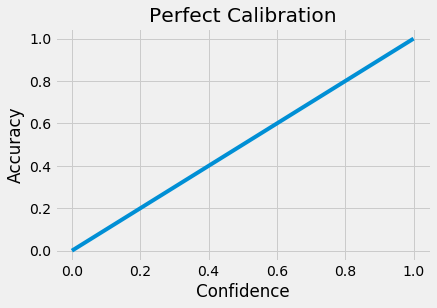
Deviance from the identity amounts to miscalibration.

Measuring Calibration

As noted in [1], “achieving perfect calibration is impossible. […] The probability in (1) cannot be computed using finitely many samples since \(\hat{P}\) is a continuous random variable.” Therefore, several statistics are designed to empirically measure a model’s calibration. In this section, we’ll summarize each method.

First, let’s define terms needed to evaluate a model given finite samples. We’ll group predictions into \(M\) bins, each of size \(1 / M\). Let \(B_m\) be the set of indices of samples whose prediction confidence falls into the interval \(I_m = (\frac{m-1}{M}, \frac{m}{M}]\), for \(m \in \{1, \dots, M\}\).

The accuracy of \(B_m\) is defined as:

The average confidence in \(B_m\) is defined as:

where \(\hat{p_i}\) is the confidence for sample \(i\).

Reliability Diagrams

Reliability diagrams are a visual tool for evaluating calibration. These diagrams plot expected sample accuracy as a function of confidence. Since perfect calibration yields the identity, any deviation represents miscalibration.

In order to calculate expected sample accuracy as a function of confidence, given finite samples, we have to first bin samples into intervals by confidence. Then, within each bin we compute the empirical accuracies and empirical confidences for the samples. Bins should have equal width to ensure plot readability.

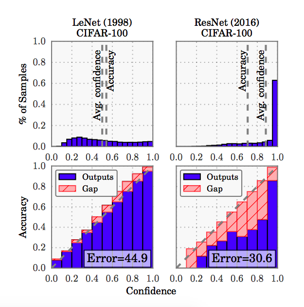
The figure above, taken from [1], shows reliability diagrams in the bottom row. We’ll discuss the meaning behind these plots in a later section.

Expected Calibration Error (ECE)

Expected Calibration Error (ECE) is the first of several calibration measures we’ll discuss that yields a scalar summary. ECE measures the difference in expected accuracy and expected confidence. Mathematically, it’s defined as:

In practice, this is computed as the weighted average of bins’ accuracy/confidence difference:

where \(n\) is the total number of samples across all bins. Perfect calibration is achieved when \(\text{ECE} = 0,\) that is \(\text{acc}(B_m) = \text{conf}(B_m)\) for all bins \(m\).

Maximum Calibration Error (MCE)

MCE is appropriate for high-risk applications, where the goal is to minimize the worst-case deviation between confidence and accuracy. Mathematically, it’s defined as:

Empirically, it’s computed as:

Cross Entropy (Negative Log Likelihood)

Cross entropy, or negative log likelihood, is not a measure of calibration but instead a standard measure of a model’s quality used often in the deep learning literature. Given a model \(\hat{\pi}(Y|X)\) and \(n\) samples, it’s defined as:

It’s shown in [2] that, in expectation, the cross entropy term is minimized if an only if \(\hat{\pi}(Y|X)\) recovers the ground truth conditional distribution \(\pi(Y|X)\)². Cross entropy is a common objective function that is minimized during training.

Modern Deep Networks are Poorly Calibrated

A key takeaway from [1] is that modern deep networks trained by minimizing a cross entropy loss are not only poorly calibrated but also less calibrated than simpler networks from the 1990s. This, counter-intuitively, comes despite substantial gains in accuracy. Figure 2 highlights the phenomenon: LeNet (1998), containing 5 layers and lacking batch-norm, has an error of 44.9% but is better calibrated than ResNet-110, containing 110 layers with batch-norm, which has an error of 30.6% on CIFAR-100. [1] proposes, and shows in the following figure, that batch-norm, increased depth and width, and weight decay all play a role affecting calibration.

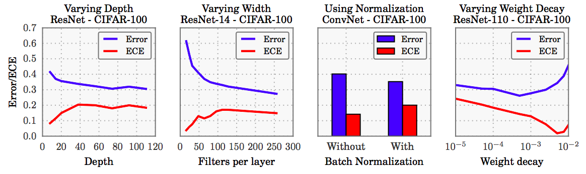
From the figure, we can see that modern developments credited with improving classification accuracy — depth, width, and batch-normalization — tend to hurt model calibration. Only weight decay (regularization) seems to improve ECE while improving accuracy.

Most interestingly, the paper highlights a disconnect between cross entropy and accuracy. They show that networks tend to overfit a cross entropy loss without overfitting to a 0/1 accuracy measure. Indeed, “surprisingly, overfitting to [negative log likelihood] is beneficial to classification accuracy. On CIFAR-100, test error drops from 29% to 27% in the region where NLL overfits. This phenomenon renders a concrete explanation of miscalibration: the network learns better classification accuracy at the expense of well-modeled probabilities.”

Importance of Calibrating your Production Model

Although the goal of solving a classification problem is to arrive at a discrete decision, models are often designed to output a probability distribution over classes. This choice is primarily motivated as a means to easily train networks. Backpropogation, the training algorithm used for neural networks, relies on the ability to differentiate the loss with respect to the network’s parameters. This requires the loss to be a smooth function of the parameters, and hence continuous in class output.

Academically, classification networks are usually judged on accuracy, as is the case with ImageNet, despite being designed to generate probability outputs. For most commercial applications of machine learning, however, probability outputs are actually desired since a classification model is usually not trained for its own sake but instead for the purpose of passing on such probabilities to some other decision-making component. In the case of a self-driving car, the system relies on an object-detection, classification model to decide if there are pedestrians in front of the car. If this predicted probability is above some threshold, the system will act as if a person is really there. The specific threshold is decided according to some risk tolerance chosen by the engineers. In this case such tolerance is probably exceptionally low. Although the object-detection model was trained to solve a classification problem, it’s not used in its capacity to pick classes. It’s merely used as a distribution-predicting mechanism. This is usually how things work in practice.

As noted earlier, there is a disconnect between minimizing a cross entropy term and being well calibrated. Because minimizing a cross entropy loss does not ensure calibration, and even tends to overfit classification accuracy, it’s imperative to calibrate any model where probabilities are passed on to some other decision making system. In practice, almost all deep models must be calibrated.

Calibration Methods

The paper highlights several techniques for performing model calibration, but for brevity we’ll only cover two: Platt scaling, which has been around for a while, and temperature scaling, which is newly proposed. Each method takes the form of an additional model that corrects the calibration error of an original model. Fitting the calibration model is a distinct, second step, done only after the original model is fully trained. Both approaches make use of a validation set (disjoint from the training set) for the purpose of fitting a calibration model.

Platt Scaling

Platt scaling applies to binary classification tasks and uses a logistic regression model to map the original network’s output probabilities to a rescaled, calibrated probability. Let \(a, b \in \mathbb{R}\) be scalar parameters. The rescaled model is \(\hat{q_i} = \sigma(az_i + b)\), where \(z_i\) is the logit for example \(i\) (the original network’s preactivation output), and \(\sigma\) is the sigmoid function: \(\sigma(x) = \frac{1}{1+e^{-x}}\). \(a\) and \(b\) are optimized using a cross entropy loss over the validation set. Note not to backprop through the original network when learning \(a\) and \(b\) since the output probabilities should be fixed.

Temperature Scaling

Temperature scaling works for classification tasks of any \(K\) by rescaling a logit vector \(z_i\) to \(\hat{q_i} = \max_k \sigma_{\text{SM}}(z_i^k / T)\). Here, \(z_i^k\) is the logit associated with sample \(i\) for class \(k\), \(T\) is a tunable temperature parameter, and \(\sigma_{\text{SM}}\) is the softmax function defined as:

\(T\) raises the output entropy when it is greater than 1. As \(T \rightarrow \infty\), \(\hat{q_i} \rightarrow 1/K\), representing maximum uncertainty. Like Platt scaling, \(T\) is trained on a cross entropy loss over validation data. Since temperature scaling performs a monotonic transformation in \(T\) of input logits, it will not affect accuracy, just confidence.

Intuitively, the temperature parameters allows us to maximize the entropy of the output distribution \(\hat{q_i}\) subject to the constraint that \(\hat{q_i}\) is still a valid probability distribution and the constraint that the average true class logit is equal to the average weighted logit. Here, “true class” is ground truth for respective validation samples used for calibration and “weighted logit” is the original network’s logit’s, \(z_i\), weighted by \(q(z_i)\), the calibrated values. The paper provides more detail into why increasing entropy is important, but in short when a model overfits to cross entropy, it tends to result in a low-entropy softmax distribution over classes. This is visible, in part, by the fact that ResNet (2016) consistently tends to have higher confidence than accuracy.

Thanks to Nishant Desai for feedback on drafts of this.